Usage

In this example we will use co2mpas_driver model in order to extract the drivers acceleration behavior as approaching the target speed.

Setup

First, set up python, numpy, matplotlib.
Set up python environment: numpy for numerical routines, and matplotlib for plotting
>>> import numpy as np >>> import matplotlib.pyplot as plt
co2mpas_driver must be imported as a dispatcher (dsp). The dsp contains functions to process vehicle data and run the com2pas_driver model. Also is necessary to import schedula for selecting and executing functions from the co2mpas_driver. For more information on how to use schedula: https://pypi.org/project/schedula/
```
>>> from co2mpas_driver import dsp
>>> import schedula as sh
```

Load data

Load vehicle data for a specific vehicle from vehicles database
```
>>> db_path = 'EuroSegmentCar.csv'
```
Load user input parameters from an excel file
```
>>> input_path = 'sample.xlsx'
```

Sample time series

>>> sim_step = 0.1 #The simulation step in seconds
>>> duration = 100 #Duration of the simulation in seconds
>>> times = np.arange(0, duration + sim_step, sim_step)

Load user input parameters directly writing in your sample script

>>> inputs = {
'vehicle_id': 35135,  # A sample car id from the database
'inputs': {'gear_shifting_style': 0.7, #The gear shifting style as
                                        described in the TRR paper
            'starting_speed': 0,
           'desired_velocity': 40,
           'driver_style': 1},  # gear shifting can take value
# from 0(timid driver) to 1(aggressive driver)
'time_series': {'times': times}
}

Dispatcher

Dispatcher will select and execute the proper functions for the given inputs and the requested outputs

>>> core = dsp(dict(db_path=db_path, input_path=input_path, inputs=inputs),
   outputs=['outputs'], shrink=True)

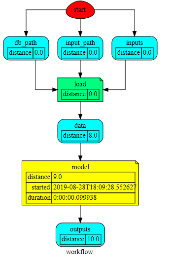
Plot workflow of the core model from the dispatcher
```
>>> core.plot()
```
This will plot the workflow of the core model on an internet browser (see below). You can click all the rectangular boxes to see in detail the sub-models like load, model, write and plot.

The Load module

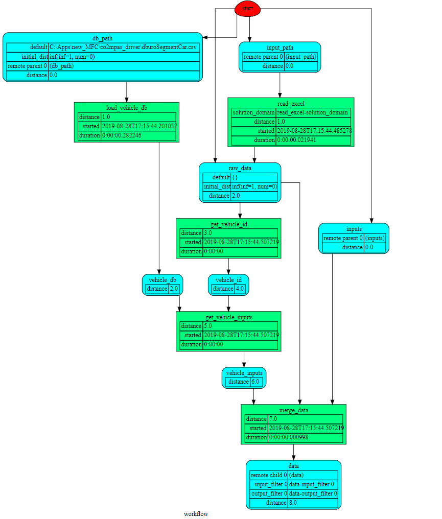
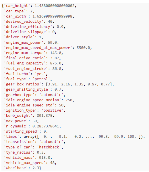
Merged vehicle data for the vehicle_id used above
Load outputs of dispatcher and select the chosen dictionary key (outputs) from the given dictionary.
```
>>> outputs = sh.selector(['outputs'], sh.selector(['outputs'], core))
```

Select the desired output

>>> output = sh.selector(['Curves', 'poly_spline', 'Start', 'Stop', 'gs',
              'discrete_acceleration_curves', 'velocities',
              'accelerations', 'transmission'], outputs['outputs'])

The final acceleration curves, the engine acceleration potential curves (poly_spline), start, stop, gear shift, discrete acceleration curves, velocities, accelerations and transmission, before calculating the resistances and the limitation due to max possible acceleration (friction).

>>> curves, poly_spline, start, stop, gs, discrete_acceleration_curves,
velocities, accelerations, transmission =
output['Curves'], output['poly_spline'], output['Start'], output['Stop'], output['gs'],
output['discrete_acceleration_curves'], output['velocities'],
output['accelerations'], output['transmission']

Plot

>>> plt.figure('Time-Speed')
>>> plt.plot(times, velocities)
>>> plt.grid()
>>> plt.figure('Speed-Acceleration')
>>> plt.plot(velocities, accelerations)
>>> plt.grid()
>>> plt.figure('Acceleration-Time')
>>> plt.plot(times, accelerations)
>>> plt.grid()

>>> plt.figure('Speed-Acceleration')
>>> for curve in discrete_acceleration_curves:
    sp_bins = list(curve['x'])
    acceleration = list(curve['y'])
    plt.plot(sp_bins, acceleration, 'k')
>>> plt.show()

Results

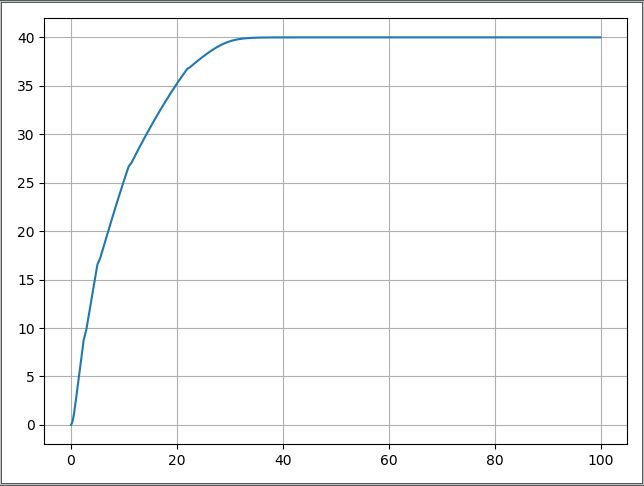
Figure 1. Speed(m/s) versus time(s) graph over the desired speed range.

Acceleration(m/s*2) versus speed(m/s) graph

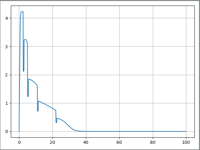
Figure 2. Acceleration per gear, the gear-shifting points and final acceleration potential of our selected vehicle over the desired speed range.

Acceleration(m/s*2) versus speed graph(m/s)

Figure 3. The final acceleration potential of our selected vehicle over the desired speed range.

Energy consumption calcultaion

From the version 1.3.3 the energy consumption calculation have been added. You can find a full example here: energy consumption example